Econometrics 463 Term Project:
The Relationship Between
Economic Freedom and Prosperity Around The World
By David Veksler
December 10, 2002
Introduction
The collapse of the Soviet Union has been followed by worldwide economic liberalization and increasing international trade. The increase in economic freedom has been followed by a global increase in prosperity, but not without setbacks. The economic slowdown beginning in the late 1990’s has caused some to question the progress of economic liberalization as well as its benefits. An analysis of relationship between economic freedom and prosperity may be useful in determining whether economic freedom increases prosperity and which specific factors have the greatest effect on wealth. This information would be very useful to anyone seeking to determine the weakness of various governmental policies. Governments may find it important to know which factors have the greatest effect on economic growth and investors may find it helpful to predict which countries are more likely to develop as potential markets.
Methodology
For this paper, ten factors that measure different aspects of economic freedom were correlated against the 2001 per capita GDP of 155 nations. There have been several studies on economic freedom since 1980 (Easton, 1997) by various think tanks. The Heritage Institute results were used for this paper because they measured the largest number of factors, and had data for over 155 countries –more than the other studies. For the GDP data, the 2001 results from the CIA Factbook were used because the CIA had the most complete and generally the latest GDP data. The Heritage Institute’s 2003 report actually came out in November 2002, but the 2001 data was used because for the majority of countries, the latest available GDP data is still for 2000 or 2001. A comparison of the Heritage Institute evaluations of economic freedom to those of the Fraser Institute (2002), showed that the reports all gave the same approximate evaluations of economic freedom.
There were ten independent variables tested: (the abbreviations used in are parenthesis)
• Trade policy (Trade)
• Fiscal burden of government (FiscalBu)
• Government intervention in the economy (Governme)
• Monetary policy (Monetary)
• Capital flows and foreign investment (ForeignI)
• Banking and finance (BK)
• Wages and prices (Wagesand)
• Property rights (Property)
• Regulation (RG)
• Black market (BlackMar)
Each of these variables was a cardinal value from one to five, with one being the least government involvement and five being the most. The dependent variable was indGDP, the 2001 per capita GDP. Additional variables considered were Econ_Sco, the overall economic score and WorldRan, the ranking according to the overall score.
Regressions were run on the overall economic score and then the ten independent variable. Initially a linear model was used, then all the variables were tested for significance under logarithmic, quadratic, and interactive relations, and variables that were not significant under any test at the 5% level were dropped from the model.
The CIA data had estimated GDP data for 236 regions -- almost every country and territory on earth, but the Heritage listed 161 countries. Of these, 155 had data available for all ten variables, so 155 countries and 10 factors were used in estimating the model. The software used for all the regressions was Gretl.
Procedure
The first step was to find out what overall relationships were present in the model. For this regression, the indGDP and Econ_Sco variables were used. A linear regression between them produced an unadjusted R-squared of 0.496862.
VARIABLE COEFFICIENT STDERROR T STAT 2Prob(t > |T|)
0) const 34622.6 2160.89 16.022 < 0.00001 ***
5) Econ_Sco -8480.91 689.958 -12.292 < 0.00001 ***
Mean of dependent variable = 8854.32
Standard deviation of dep. var. = 9169.89
Sum of squared residuals = 6.51533e+009
Standard error of residuals = 6525.63
Unadjusted R-squared = 0.496862
Adjusted R-squared = 0.493573
A more closer match was found by adding sq_Econ to the model:
VARIABLE COEFFICIENT STDERROR T STAT 2Prob(t > |T|)
0) const 76270.6 5767.89 13.223 < 0.00001 ***
5) Econ_Sco -36958.0 3782.94 -9.770 < 0.00001 ***
17) sq_Econ_ 4575.07 600.351 7.621 < 0.00001 ***
Mean of dependent variable = 8854.32
Standard deviation of dep. var. = 9169.89
Sum of squared residuals = 4.71419e+009
Standard error of residuals = 5569.06
Unadjusted R-squared = 0.635953
Adjusted R-squared = 0.631163
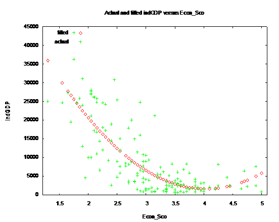
The graph below shows the predicted model and the Econ_Sco variables:

The relationship here is clear: increasing government involvement lowers GDP at a rate of $36, 958 per index point. The quadratic function seems to indicate that super-high levels of involvement actually raise GDP, but only about six countries seem to be part of that trend, with two having a per capita GDP above 5000: Iran and Libya.
After a simple one-factor regression, a regression with all ten factors (but not Econ_Sco) was attempted. Initially, a simple linear regression was used with all 155 variables and all 10 factors, without any quadratic or interacting variables:
VARIABLE COEFFICIENT STDERROR T STAT 2Prob(t > |T|)
0) const 20847.5 2372.98 8.785 < 0.00001 ***
6) Trade -1209.12 445.846 -2.712 0.007503 ***
7) FiscalBu 1576.36 481.540 3.274 0.001330 ***
8) Governme 976.563 594.194 1.644 0.102459
9) Monetary -609.650 333.642 -1.827 0.069732 *
10) ForeignI 194.577 720.675 0.270 0.787553
11) BK -826.296 689.728 -1.198 0.232884
12) Wagesand 1382.06 720.518 1.918 0.057071 *
13) Property -2068.62 739.690 -2.797 0.005870 ***
14) RG -213.362 838.028 -0.255 0.799395
15) BlackMar -2863.18 535.661 -5.345 < 0.00001 ***
Mean of dependent variable = 8854.32
Standard deviation of dep. var. = 9169.89
Sum of squared residuals = 3.43621e+009
Standard error of residuals = 4884.93
Unadjusted R-squared = 0.734643
Adjusted R-squared = 0.716216
F-statistic (10, 144) = 39.8665 (p-value < 0.00001)
Durbin-Watson statistic = 2.14011
First-order autocorrelation coeff. = -0.071209
(Higher coefficients indicate higher government involvement in the various areas.)
A test for quadratic variables was used:
VARIABLE COEFFICIENT STDERROR T STAT 2Prob(t > |T|)
0) const 25616.2 5818.15 4.403 0.000022 ***
6) Trade 3241.39 1794.43 1.806 0.073105 *
7) FiscalBu -4843.72 2560.55 -1.892 0.060693 *
8) Governme 596.296 2228.13 0.268 0.789402
9) Monetary -263.771 1262.99 -0.209 0.834885
10) ForeignI -867.630 2083.24 -0.416 0.677725
11) BK -2086.66 1858.50 -1.123 0.263547
12) Wagesand -2955.80 2517.71 -1.174 0.242476
13) Property -3070.39 1991.59 -1.542 0.125510
14) RG -1281.77 2795.31 -0.459 0.647305
15) BlackMar -7242.81 1796.90 -4.031 0.000093 ***
16) sq_Trade -423.008 265.461 -1.593 0.113407
17) sq_Fisca 744.970 378.890 1.966 0.051343 *
18) sq_Gover -149.109 386.857 -0.385 0.700524
19) sq_Monet 121.290 207.138 0.586 0.559160
20) sq_Forei 88.0300 369.384 0.238 0.812000
21) sq_BK 338.051 314.633 1.074 0.284561
22) sq_Wages 216.479 414.127 0.523 0.602022
23) sq_Prope 626.785 334.349 1.875 0.063019 *
24) sq_RG 135.053 428.646 0.315 0.753199
25) sq_Black 1210.16 262.880 4.603 < 0.00001 ***
Unadjusted R-squared = 0.396284
Adjusted R-squared = 0.306177
Test statistic: TR^2 = 61.424005,
with p-value = prob(Chi-square(10) > 61.424005) = 0.000000
And a test for logs:
VARIABLE COEFFICIENT STDERROR T STAT 2Prob(t > |T|)
0) const -1873.56 2260.44 -0.829 0.408665
6) Trade -1990.24 1334.03 -1.492 0.138075
7) FiscalBu 4059.26 2287.05 1.775 0.078187 *
8) Governme -506.908 1945.41 -0.261 0.794827
9) Monetary 804.378 1058.59 0.760 0.448676
10) ForeignI 192.145 1865.56 0.103 0.918120
11) BK 1984.84 1670.56 1.188 0.236883
12) Wagesand 847.905 2099.09 0.404 0.686902
13) Property 3116.16 1779.32 1.751 0.082179 *
14) RG 343.683 2304.40 0.149 0.881666
15) BlackMar 6442.66 1340.24 4.807 < 0.00001 ***
17) l_Trade 6925.99 3734.78 1.854 0.065872 *
18) l_Fiscal -12569.4 7106.97 -1.769 0.079236 *
19) l_Govern 978.852 4892.75 0.200 0.841736
20) l_Moneta -960.438 2574.34 -0.373 0.709678
21) l_Foreig -1249.52 4273.17 -0.292 0.770425
22) l_BK -4921.49 3858.68 -1.275 0.204362
23) l_Wagesa -6570.98 5447.23 -1.206 0.229828
24) l_Proper -6491.89 4115.55 -1.577 0.117061
25) l_RG -2554.60 6290.98 -0.406 0.685337
26) l_BlackM -16450.3 3732.15 -4.408 0.000021 ***
Unadjusted R-squared = 0.411176
Adjusted R-squared = 0.323292
Test statistic: TR^2 = 63.732241,
with p-value = prob(Chi-square(10) > 63.732241) = 0.000000
It appears that sq_Fisca, sq_Prope, sq_Black, and l_Trade and l_BlackM are significant, so these variables were created:
Model 2: OLS estimates using the 155 observations 1-155
Dependent variable: indGDP
VARIABLE COEFFICIENT STDERROR T STAT 2Prob(t > |T|)
0) const 34351.3 9683.62 3.547 0.000531 ***
6) Trade -2750.11 1190.66 -2.310 0.022376 **
7) FiscalBu -2757.13 2424.35 -1.137 0.257385
8) Governme 964.732 488.511 1.975 0.050267 *
9) Monetary -109.990 271.083 -0.406 0.685555
10) ForeignI -190.634 582.886 -0.327 0.744120
11) BK -965.605 556.143 -1.736 0.084735 *
12) Wagesand -63.7690 603.954 -0.106 0.916063
13) Property -5953.28 1787.79 -3.330 0.001112 ***
14) RG -867.724 679.755 -1.277 0.203899
15) BlackMar 1615.02 9421.44 0.171 0.864143
16) l_Trade 5907.95 3327.77 1.775 0.078029 *
17) l_BlackM -15172.6 11337.6 -1.338 0.182998
18) sq_Fisca 651.370 362.476 1.797 0.074507 *
19) sq_Prope 800.209 284.262 2.815 0.005586 ***
20) sq_Black 233.137 848.323 0.275 0.783861
Mean of dependent variable = 8854.32
Standard deviation of dep. var. = 9169.89
Sum of squared residuals = 2.08499e+009
Standard error of residuals = 3872.98
Unadjusted R-squared = 0.838989
Adjusted R-squared = 0.821614
F-statistic (15, 139) = 48.2863 (p-value < 0.00001)
Durbin-Watson statistic = 1.84585
First-order autocorrelation coeff. = 0.0767549
Taking out the non-significant variables, the resulting regression is:
Model 3: OLS estimates using the 155 observations 1-155
Dependent variable: indGDP
VARIABLE COEFFICIENT STDERROR T STAT 2Prob(t > |T|)
0) const 31596.2 2336.61 13.522 < 0.00001 ***
6) Trade -2970.81 1199.32 -2.477 0.014387 **
8) Governme 756.926 481.722 1.571 0.118279
11) BK -1047.66 493.696 -2.122 0.035519 **
13) Property -8954.56 1615.13 -5.544 < 0.00001 ***
16) l_Trade 6379.73 3351.79 1.903 0.058959 *
17) l_BlackM -7828.71 1176.19 -6.656 < 0.00001 ***
18) sq_Fisca 242.486 56.5346 4.289 0.000032 ***
19) sq_Prope 1273.94 249.607 5.104 < 0.00001 ***
Mean of dependent variable = 8854.32
Standard deviation of dep. var. = 9169.89
Sum of squared residuals = 2.3127e+009
Standard error of residuals = 3980
Unadjusted R-squared = 0.821405
Adjusted R-squared = 0.811619
F-statistic (8, 146) = 83.9364 (p-value < 0.00001)
Durbin-Watson statistic = 1.97101
First-order autocorrelation coeff. = 0.0129411
Government and log(Trade) do not appear to be significant in this model, so they were dropped:
VARIABLE COEFFICIENT STDERROR T STAT 2Prob(t > |T|)
0) const 32948.4 2093.65 15.737 < 0.00001 ***
6) Trade -701.47 352.948 -1.987 0.048715 **
11) BK -930.70 492.710 -1.889 0.060856 *
13) Property -9310.0 1571.14 -5.926 < 0.00001 ***
18) l_BlackM -7606.7 1174.58 -6.476 < 0.00001 ***
19) sq_Fisca 255.859 56.3419 4.541 0.000012 ***
20) sq_Prope 1329.27 242.992 5.470 < 0.00001 ***
Mean of dependent variable = 8854.32
Standard deviation of dep. var. = 9169.89
Sum of squared residuals = 2.40055e+009
Standard error of residuals = 4027.4
Unadjusted R-squared = 0.814621
Adjusted R-squared = 0.807105
F-statistic (6, 148) = 108.394 (p-value < 0.00001)
Durbin-Watson statistic = 2.01359
First-order autocorrelation coeff. = -0.00986223
The estimated model was thus:
indGDP=32948.4 -701.47 *Trade -930.70 BK--9310.0 *Property-7606.7 *log(BlackM)+ 255.859 *Fiscal^2 + 1329.27 *Property^2
(The mean of indGDP was 8854.323 and S.D. was 9169.893 , and the mean of Econ_Sco was 3.0384 and S.D. of 0.76215.)
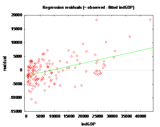
Below are the observed versus fitted ingGDP residuals:

Summary and Discussion
The most obvious evidence shown by the data is that the average value of economic freedom has a strong relationship with per capita GDP. The R-squared value in the quadratic model with Econ_Sco is 0.635953 and at least up to a freedom factor of about 4.2, where the trend suddenly reverses. This may be because the three outliers at the 4.5 range (Libya (capita GDP of 7600) Iran (capita GDP of 6400), and Iraq (capita GDP of 2500)) are socialist economies that maintain unusually high incomes because they derive most of their GDP from oil exports. However, the quadratic relation also suggests that increasing government involvement is progressively less harmful to indGDP. On the other hand, this also means that decreasing government involvement is exponetial more beneficial to GDP.
The final model derived from the regressions was:
indGDP=32948.4 -701.47 *Trade -930.70 BK--9310.0 *Property-7606.7 *log(BlackM)+ 255.859 *Fiscal^2 + 1329.27 *Property^2
This model has several interesting properties. First, it is surprisingly accurate at predicting per capita GDP. With an R-squared of 0.814621, it indicates that 81 percent of variation in wealth between countries is caused by their economic policies. This makes the fact that increased economic freedom leads to more prosperity is hard to dispute. The model also shows that other than the small positive coefficient on fiscal burden, there are strong negative correlations between the above factors and prosperity: that is, free trade, strong property rights, and low black market activity lead to higher prosperity. The question of what exact effect the factors had on GDP and which factors were most influences was more complicated however.
The BlackM factor, or the amount of black market activity shows a high negative, suggesting that the more market activity is conducted underground, the lower the level of GDP. This is highly intuitive, as illegal and hidden activities are bound to have significantly higher costs because of the usual costs risk associated with operating against the law. These factors may be a good proxy for how difficult it is to run a business legally in any given country. Of course when a large percentage of business is underground, most of the legal restrictions on businesses do not apply, which may diminish the accuracy of the other variables at high levels of black market activity. There are 45 countries with the highest level of black market activities, with an average economic freedom ranking of about 124, and average capita GDP of $2,746, significantly below the world average of $8,854.
Trade was another major factor. The quadratic relationship suggests that increasing free trade yields diminishing returns, but the overall pattern was clear: the 34 nations with the highest level of trade restrictions have a capita GDP of $3,578.53 and the top eight nations with the highest level of trade freedom have an average capita GDP of $11,577.5. Since the grading system uses cardinal rather than quantitative rankings, it was hard to get more precise estimates of the effect of trade restrictions, but free trade nevertheless seems to be an important factor for GDP growth. Economic theory would suggest this outcome, since foreign investment is key in the growth of developing nations. A time series study on the growth in GDP versus trade restrictions may clarify this theory.
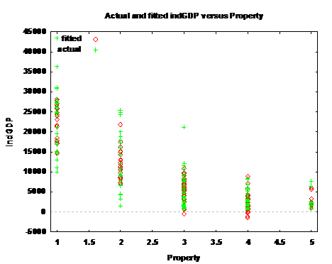
Property rights had the biggest coefficient out of all the other factors, which is not at all surprising, considering that private property ownership is at the root of capitalism. However the relationship was not linear, as the plot of the actual and fitted indGDP versus Property bellow shows:

Despite the non-linear relationship, the trend in the quadratic relationship reverses itself only in unfree countries, which may be an indication that property rights are less effective in nations that already have weak property rights protections. Indeed, the average per capita income in the 14 nations with the lowest level of property rights is $2,563.08 and their average ranking is only 144.6 out of 155.
An unexpected result of the model was that increasing fiscal burden (which is defined as “tax rates and the level of government expenditures” (Heritage p53)) seems to actually raise per capita GDP. This may be explained by the fact that as nations get wealthier, increasing profits allow higher taxes to be raised. Nevertheless, taxes do not seem to have a significant impact on GDP, and are probably not the first thing a country should look to cut if it desires economic growth
It is unclear why a number of variables (like foreign investment) that are clearly significant individually were not significant in the full model. When a regression was done on the individual variables, nearly all (other than fiscal burden) variables show significant negative correlations between more government and per capita GDP. This suggests that there is some degree of collinearity in the variables, which is not surprising considering that each factor attempts to isolate certain aspects of bureaucratic policy from a single structure of regulation.
While the particular relationship between the ten factors used is less than clear, the basic conclusion from the data is beyond question: increasing levels of economic freedom are highly correlated with increasing levels of per capita GDP, and the variation in economic freedom explains most of the differences in wealth around the world. This outcome would be surprising to many individuals who attribute factors like natural resources, population growth, or income distributions to differences in wealth, and holds many lessons for anyone attempting to stimulate growth in their own country or companies looking for growth opportunities around the world.
References
1. Easton, S. T., and Walker, M.A., eds. (1992) Rating Global Economic Freedom. Vancouver, B.C., Canada: The Fraser Institute.
2. Hanke, S.H., and Walters, S.J.K. (1997) Liberty, Equality, Prosperity. A Report to the Senate Joint Economic Committee. Washington, D.C.: U.S. Senate.
3. Gerald P. O’Driscoll, Jr., Kim R. Holmes, (2002) 2002 Index of Economic Freedom. Washington, D.C.: The Heritage Foundation.
3. Gerald P. O’Driscoll, Jr., Edwin J. Feulner, (2002) 2003 Index of Economic Freedom. Washington, D.C.: The Heritage Foundation.
4. CIA World Factbook 2002.
http://www.cia.gov/cia/publications/factbook/
5. Economic Freedom of the World, 2000. (2002) Fraser Institute.
6. Gwartney, James, and Lawson, Robert. Capital University Economic Freedom of the World Annual Report 2002: Cato Institute.
http://www.cato.org/economicfreedom